| In this paper, we describe a new straight line detection algorithm, using derivative-based edge operators, which works without internal thresholding nor any internal parameterization (see below). It has been presented in the Third Workshop on Electronic Control and Measuring Systems, Université Paul Sabatier (Toulouse), on June 2-3, 1997. Although minor modifications have occur, the version presented here is a copy of the version published in the proceedings, a French version is available. | |
PDF version here | |
| |
In this paper, we describe a new straight line detection algorithm, using derivative-based edge operators, which works without internal thresholding nor any internal parameterization. This property delays the detection decisions up to the high levels of the image analysis system rather than in the low level line detection processes. This reduces the amount of parameters to adjust in the supervising image understanding system. This method also allows low contrast lines to be detected, without an excess of false alarms, because the spurious isolated noise pixels marked as edges in the first phases will not be validated in the following phases. The method is mostly based upon simple filter computations which should be able to produce fast results in hardware embodiment.
Line-detection algorithms based on contour extraction usually involve the following stages of image processing: smoothing, edge detection, edge thinning, edge linking, chain straightening and line correction. In our algorithm, the second stage includes two derivative processes using well-known laplacian and gradient filters [WANG94] to determine edge location and orientation. The three last stages process the lines extraction. The above-mentioned smoothing and thinning stages known from literature are not processed as they are implicit in the algorithm by the choice of the derivative method.
The algorithm is thus executed in 5 phases : edge detection, edge direction computation, edge linking, chain straightening and line restoration.
In phase 1, thin edges are detected on zero crossings of the laplacian convolution filter's response. The filter used is the sum of the second derivative one-dimensional filters in either 2 or 4 directions (using diagonals). The size of the laplacian filter determines the bandwidth of the implicit smoothing in the filter process.
The White-Rohrer (two directions, [WHIT83]) and Marr-Hildreth (four directions, [HARA84]) filters use the matrixes MWR and MMH (equations 1 and 2).
 (1),
(1), ![Laplacian 3×3 : [L=(1 -2 1)] L+L'+rot(L,45°)+rot(L',45°)](eq2.gif) (2)
(2)
 (4)
(4)
The figures 1 and 2 represent the response on White-Rohrer (fig. 1) and Marr-Hildreth (fig. 2) filter in a zone where edgels were present ; the figures 3 and 4 represent the same filters responses in a no-edgels zone. The intensities have been corrected to present the same noise levels in both filters (the noise measurement is the standard deviation of the no-edgels samples). Comparing intensities of laplacian response on edgel zone versus average response on non-edgel zone, taking the correction into account, the signal-to-noise ratio is better on the Marr-Hildreth filter than on the White-Rohrer one.
|
|
| figure 1 : laplacian (White-Rohrer filter with correction) | figure 2 : laplacian (Marr-Hildreth filter) |
 measured standard deviation : 7.62 |
 measured standard deviation : 7.59 |
| figure 3 : noise sample (White-Rohrer with correction) | figure 4 : noise sample (Marr-Hildreth) |
Zero-crossings of the laplacian represent inflection points in the direction of the gradient of the image (which is a R² to R function). However, some inflection points of the image do not represent edges. This occurs ([FLEC92]) where the sign of the first derivative is the same as the sign of the third derivative. This may be demonstrated on examples on R to R functions that will be continuously derivable in the neighbourhood of the considered point.
To be declared as edge, an inflection point requires the following conditions :
In these two cases, the sign of f' is different from the sign of f''' . In the other two cases (fig. 5.b and 5.d), the inflection point does not belong to an edge.
|
|
| figure 5.a : f increasing with a local maximum of f' | figure 5.b : f increasing with a local minimum of f' |

|
|
| figure 5.c : f decreasing with a local minimum of f' | figure 5.d : f decreasing with a local maximum of f' |
The usual thinning phase of chain extraction algorithms is not needed here because the zero-crossing of the laplacian delivers thin edges. However, neighbouring edges in gradient direction may appear [TORR86] when anti-parallel boundaries are one pixel apart, or when the algorithm associates vertical and horizontal zero-crossing edges around a corner.
2.2 Edge direction computation
In phase 2, the orientation of each detected edge is computed by 2 directional gradient filters (vertical and horizontal) which estimate the 2 coordinates of the gradient vector. The matrixes used and the derivation operations are shown on equations 5 et 6.
Vertical component : ![]() ,
, ![]() (5),
(5),
Horizontal component :![]() ,
, ![]() (6)
(6)
These operators are not very accurate for localisation purposes. One can notice it on figures 6 and 7 which represent responses from edge detection by these filters (fig. 6) and the White-Rohrer laplacian (fig. 7). These are thus not very efficient for edge detection.
|

|
| Figure 6 : edge detection by 2-component gradient | Figure 7 : edge detection by laplacian |

|
| Figure 8 : edge and gradient |
The gradient direction will not need to be known with a great precision, as it is only used to resolve 8-pixel neighbouring in the link process in the next phase. The gradient direction is represented with one of the 8 possible directions from the central pixel ; this leads to a 3 bits storage, and a maximum error of 22.5° (figure 9).
|
| Figure 9 : Representation of the 8 direction classes |
Whereas an edge occurs between two pixels, the edge is set on the pixel that presents the weakest intensity (the darkest). The null-intensity edges are not represented. The intensity and direction is shown for every edge. The length of the arrow is proportional to the intensity of the edge. The direction of the edge has been represented with doted lines and fixed length for some pixels.

|

|
| Figure 10 : zoom on a corner in an image | Figure 11 : directions and intensities of gradient in the same zone |
The next pixel will be theta because this one is one of the three eligible successors of epsilon (which are dzeta, iota et theta), epsilon is one of the three eligible predecessors of theta (which are epsilon, delta and eta), and the edge directions of pixels epsilon and theta are the same.
This chaining is not relevant in case of neighbouring edges in gradient direction which indicates aggregated anti-parallel boundaries in high frequency textured pictures. The edge map needs a non-maximum edge suppression before phase 3 is processed in order to reduce the image's texture frequency and sample the edges to deliver to the next phase. The non-maximum suppression of edges removes the edgels which present an edgel of weakest intensity next to them (in a direction orthogonal to their own direction). For each edgel pe, the edge intensities of its side neighbours (in the direction of its gradient) is computed. If one of these two neighbours has its intensity greater than pe,'s intensity, then pe, is removed from the edge map. Actually, few edgels will be removed by this process.
An example of the non-maximum edge suppression process is presented on figures 12 and 13: a zoom on an image around a corner (fig. 12), and the directions and intensities of its edges (fig. 13). The corner edgel (of intensity 164) has a neighbour in its gradient direction, which presents an edge of highest intensity (204). The corner edgel will be removed.

|
|
| Figure 12 : zoom on a corner in an image | Figure 13 : directions and intensities of gradient in the same zone |

|
| Figure 14 : straightening of a chain |
Some lines produced by phase 4 somehow misfit the actual lines of the image. The main cause is corner splitting. Since thin edges are used, an edgel cannot have more than two neighbours. Only edgels which present continuous variation in their direction are linked together. For these two reasons, an edge chain cannot contain an angle greater than 45°. It may also appear that a corner is split due to weak contrast or high frequency noise in the picture.
The corner dislocation does not interfere on a critical basis with our purpose which focus on images that present a bi-level intensity distribution, based upon binary images in the significant area. In this kind of images, lines intersections cannot occur. The restoration phase used here is sufficient for our aim.
Figures 16 and 17 present the lines extracted from figure 15 with and without lines restoration. The set of line is more consistent after the restoration phase, even if some defects are not actually visible. On figure 16, the lines on the left of the Data-Matrix symbol (in the centre of the image) are shown as two joint orthogonal lines. They are actually separated, and have their extremities lying on neighbouring pixel (of exactly one pixel apart) which appear as one consistent corner. The line which is indicated by a light arrow in picture 17 appears to be broken in the picture 16 and is corrected by the restoration phase.

|
|
| Figure 15 : image containing straight lines | Figure 16 : raw line extraction from figure 15 |
|
|
| Figure 17 : restored lines from figure 16 (superimposed on original image) |
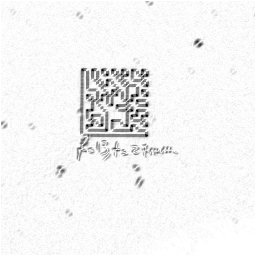
The method has been designed for the detection process of bi-level bar-codes derivatives in pictures. (Data-Matrix codes are shown on figures 15 and 18). These symbol are printed on a bi-level basis, and attained by way of camera in real-world situation, which include optic and projective distortion, unreliable lighting... The aim of the process is to detect and localise the symbol.
The method delivers multiple little linked lines as response from a curvature boundary, which results in the polygonization of the objects' boundary ; if this may be a handicap for some image understanding processes, it does not affect our objective. Indeed, the symbol is composed of shapes with straight borders ; the shapes and texture characteristics of areas outside the symbol are of no interest, and the way that our line detector reacts on these textures does not concern us for this application as long as it cannot be misinterpreted as symbol characteristics (which are long lines).
The symbol is itself a bi-level pattern, which means that it can be represented unambiguously by a set of shapes, or by a set of closed thin boundaries representing these shapes. This characteristic implies that the original picture, in the area where the symbol stands, does not contain no-edge inflection points, nor wide edges with uncertain localisation, nor vertex or line extremities where chain linking could not be solved unambiguously. The derivation process used (zero-crossing of the laplacian which naturally produces thin closed boundaries) as well as the non-maximum edge suppression and the iterative linking process may produce spurious or missing edge element, but these hindrances barely occurs in our application field.
As we have explained in § 2.5, our methods induces corner dislocation which is corrected by the restoration phase. As symbol images do not contain lines intersecting, disjoint lines on corner of symbol shapes are properly recovered by the restoration phases.
These detectors are to be implemented in human-usable devices which need fast calculation. As several of this method's phases are based upon linear filter operators, fast processing of the low level phases should be achieved using proper hardware implementation.
However, the method does not work well on little lines (2 to 3 pixels). These lines cannot be properly constructed out of responses from filters of size 2×2 or 3×3, and are irrevocably lost as edge-location errors induce some significant errors in the line directions. As a consequence, the short line elimination of phase 3 does not depreciate the final detection results as short lines were unreliably detected anyway.
Figures 18 to 20 present the result of the detection process on Data Matrix images.
|
|
| Figure 18 : image of a Data-Matrix symbol | Figure 19 : line detection result |
|
|
| Figure 20 : line detection result superimposed on image 18 |